Mathematik-Online-Aufgabensammlung: Lösung zu: Aufgabe 1364: Ein inhomogenes System linearer Differentialgleichungen

	[Home] [Lexikon] [Aufgaben] [Tests] [Kurse] [Begleitmaterial] [Hinweise] [Mitwirkende] [Publikationen]
	Mathematik-Online-Aufgabensammlung: Lösung zu
	Aufgabe 1364: Ein inhomogenes System linearer Differentialgleichungen

A B C D E F G H I J K L M N O P Q R S T U V W X Y Z

Es seien

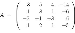
$\begin{displaymath} A \; =\; \left( \begin{array}{rrrr} 3 & 5 & 4 &-14 \\ 1 ... ... \\ -2 &-1 &-3 & 6 \\ 1 & 2 & 1 & -5 \\ \end{array}\right) \end{displaymath}$

und

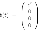
$\begin{displaymath} b(t) \; =\; \left( \begin{array}{c} e^t \\ 0 \\ 0 \\ 0 \\ \end{array}\right)\; . \end{displaymath}$

Bestimme die allgemeine Lösung von $\dot{u}(t) = A u(t) + b(t)$ .

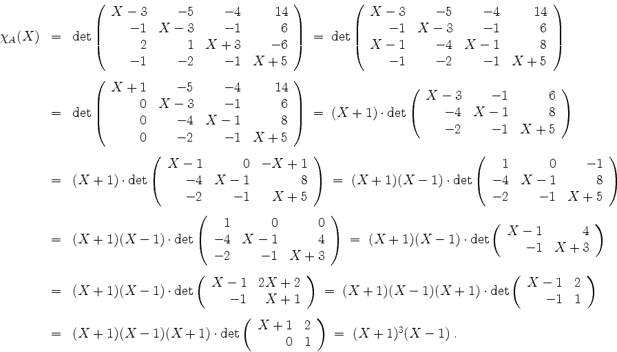
Es wird

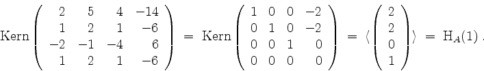
$\begin{displaymath} \begin{array}{rcl} \chi_A(X) & = & \det\left( \begin{array}... ... \end{array} \right) \; =\; (X+1)^3(X-1) \; . \\ \end{array}\end{displaymath}$

Beim Eigenwert erhalten wir

$\begin{displaymath} \mathrm{Kern}\left( \begin{array}{rrrr} 2 & 5 & 4 &-14 \\ ... ... 1 \\ \end{array}\right) \rangle \; = \; \mathrm{H}_A(1) \; . \end{displaymath}$

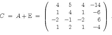
Beim Eigenwert setzen wir zunächst

$\begin{displaymath} C \; =\; A + \mathrm{E} \; = \; \left( \begin{array}{rrrr} ... ... -2 &-1 &-2 & 6 \\ 1 & 2 & 1 & -4 \\ \end{array}\right)\; . \end{displaymath}$

Wir erhalten

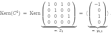
$\begin{displaymath} \mathrm{Kern}(C^1) \; = \; \mathrm{Kern}\underbrace{\left( ... ... 1 \\ 0 \\ \end{array}\right)}_{=:\; y_{1,1}} \rangle \; . \end{displaymath}$

Ferner wird

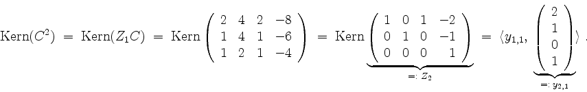
$\begin{displaymath} \mathrm{Kern}(C^2) \; = \; \mathrm{Kern}(Z_1 C) \; = \; \ma... ... 0 \\ 1 \\ \end{array}\right)}_{=:\; y_{2,1}} \rangle \; . \end{displaymath}$

Schließlich wird

$\begin{displaymath} \mathrm{Kern}(C^3) \; = \; \mathrm{Kern}(Z_2 C) \; = \; \ma... ...y}\right)}_{=:\; y_{3,1}} \rangle \; = \; \mathrm{H}_A(-1)\; . \end{displaymath}$

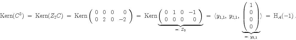
Wählen wir $x_{3,1} := y_{3,1}$ , so sind schon aus Dimensionsgründen in den Stufen und keine weiteren Vektoren auszuwählen. Der Eigenwert liefert also die Kette

$\begin{displaymath} (C^2 x_{3,1}, C x_{3,1}, x_{3,1}) \; = \; (\left( \begin{ar... ...egin{array}{r} 1 \\ 0 \\ 0 \\ 0 \\ \end{array}\right)) \end{displaymath}$

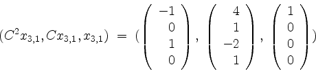
als Beitrag zur Matrix

Insgesamt erhalten wir mit

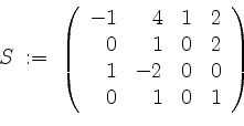
$\begin{displaymath} S \; :=\; \left( \begin{array}{rrrr} -1 & 4 & 1 & 2 \\ 0 ... ...2 \\ 1 &-2 & 0 & 0 \\ 0 & 1 & 0 & 1 \\ \end{array}\right) \end{displaymath}$

die Jordanform

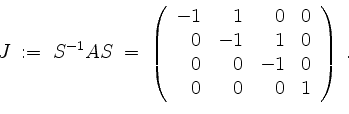
$\begin{displaymath} J \; :=\; S^{-1} A S \; = \; \left( \begin{array}{rrrr} -1 &... ... 0 & 0 &-1 & 0 \\ 0 & 0 & 0 & 1 \\ \end{array}\right)\; . \end{displaymath}$

Somit erhalten wir

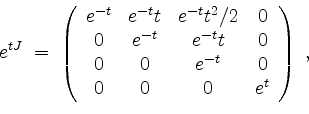
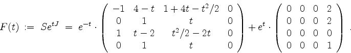
$\begin{displaymath} e^{tJ} \; = \; \left( \begin{array}{cccc} e^{-t} & e^{-t}t... ...0 & e^{-t} & 0 \\ 0 & 0 & 0 & e^t \\ \end{array}\right)\; , \end{displaymath}$

also für die allgemeine Lösung der zugehörigen homogenen Differentialgleichung die Fundamentalmatrix

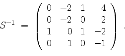
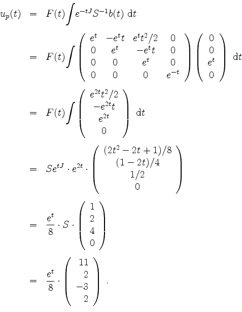
$\begin{displaymath} F(t) \; := \; S e^{tJ} \; = \; e^{-t}\cdot \left( \begin{ar... ... 0 & 0 & 0 & 0 \\ 0 & 0 & 0 & 1 \\ \end{array}\right) \; . \end{displaymath}$

Bestimmen wir nun eine partikuläre Lösung der inhomogenen Gleichung. Hierzu berechnen wir zunächst

$\begin{displaymath} S^{-1} \; = \; \left( \begin{array}{rrrr} 0 & -2 & 1 & 4 \\... ... 1 & 0 & 1 & -2 \\ 0 & 1 & 0 & -1 \\ \end{array}\right)\; . \end{displaymath}$

Sodann wird die partikuläre Lösung

$\begin{displaymath} \begin{array}{rcl} u_p(t) & = & F(t) {\displaystyle\int} e^{... ... 2 \\ -3 \\ 2 \\ \end{array}\right) \; . \\ \end{array}\end{displaymath}$

Somit ist die allgemeine Lösung von der Form

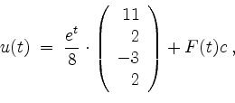
$\begin{displaymath} u(t) \; = \; \dfrac{e^t}{8}\cdot \left( \begin{array}{r} 11 \\ 2 \\ -3 \\ 2 \\ \end{array}\right) + F(t) c\; , \end{displaymath}$

wobei

wie oben beschrieben sei, und wobei $c\in\mathbb{C}^4$ ein beliebig wählbarer Vektor ist.

(Autoren: Künzer/Martin/Tentler/Wahrheit)

[Zurück zur Aufgabe]

automatisch erstellt am 11. 8. 2006