
Mathematik-Online-Lexikon:
|
|
[Home] [Lexikon] [Aufgaben] [Tests] [Kurse] [Begleitmaterial] [Hinweise] [Mitwirkende] [Publikationen] |
|
Mathematik-Online-Lexikon: | |
Ein System von linearen Differentialgleichungen mit Anfangswertproblem |
| A B C D E F G H I J K L M N O P Q R S T U V W X Y Z | Übersicht |
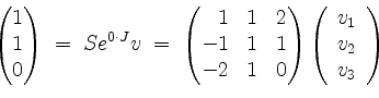
Sei
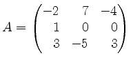 .
.
Lösung.
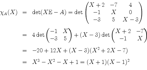
Also hat
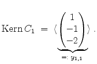
Dies ist eine Basis des Hauptraums
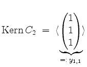
sowie
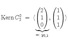
woraus wir eine Basis
Wir ersetzen nun im nächsten Schritt diese Basis durch die einzige hier erforderliche Kette
![]() , welche ebenfalls eine Basis des Hauptraums
, welche ebenfalls eine Basis des Hauptraums
![]() darstellt.
(Daß
darstellt.
(Daß
![]() ist, darf als Zufall angesehen werden.) Insgesamt erhalten wir
ist, darf als Zufall angesehen werden.) Insgesamt erhalten wir
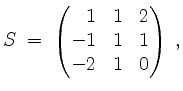
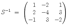
und es ist
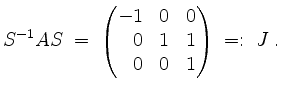
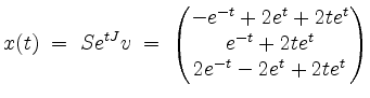
Dann ist also
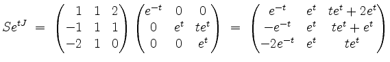
eine Fundamentalmatrix, so daß die allgemeine Lösung der Differentialgleichung die Gestalt
hat, mit einem Vektor
und daraus die eindeutige Lösung
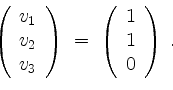
Somit ist
die eindeutige Lösung des gegebenen Anfangswertproblems.
mit einem noch zu bestimmenden
Wir berechnen zunächst
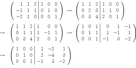
Also ist
und
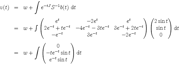
mit einem konstanten Vektor
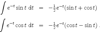
Daraus erhält man mit partieller Integration
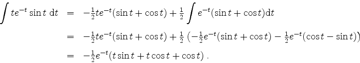
Somit ist
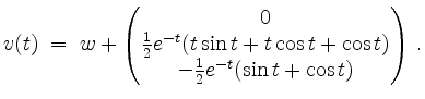
Die allgemeine Lösung ist demnach
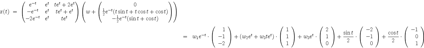
mit einem Vektor
| automatisch erstellt am 22. 8. 2006 |