Mathematik-Online-Kurs: Analysis einer Veränderlichen - Differentiation - Taylor-Entwicklung
|
|
[Home] [Lexikon] [Aufgaben] [Tests] [Kurse] [Begleitmaterial] [Hinweise] [Mitwirkende] [Publikationen] |
|
Mathematik-Online-Kurs: Analysis einer Veränderlichen - Differentiation - Taylor-Entwicklung | |
Taylor-Polynom |
| [vorangehende Seite] [nachfolgende Seite] | [Gesamtverzeichnis][Seitenübersicht] |
Direktes Nachrechnen zeigt die Übereinstimmung
der Ableitungen von ![]() und
und ![]() .
.
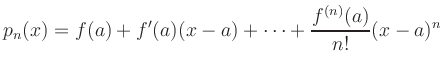
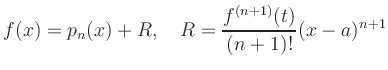
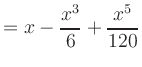
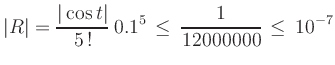
Zur Überprüfung des Restglieds ![]() ergänzt
man das Taylor-Polynom um einen weiteren Term:
ergänzt
man das Taylor-Polynom um einen weiteren Term:
 |
||
 |
||
 |
Entsprechend gilt für die Kosinusfunktion
 |
||
 |
||
 |
![\includegraphics[height=4.5cm]{Taylor_sin}](/inhalt/beispiel/beispiel137/img23.png) |
![\includegraphics[height=4.5cm]{Taylor_cos}](/inhalt/beispiel/beispiel137/img24.png) |
Wie aus der Abbildung ersichtlich ist, wird die Approximation für großes ![]() erst bei höheren Graden hinreichend genau. In der Tabelle sind die Fehler für einige
erst bei höheren Graden hinreichend genau. In der Tabelle sind die Fehler für einige ![]() -Werte angegeben.
-Werte angegeben.
| 3.1416 | 0.5708 | 0.1812 | 0.0783 | 0.0405 | 0.0236 | |
| 2.0261 | 0.0752 | 0.0102 | 0.0025 | 0.0008 | 0.0003 | |
| 0.5240 | 0.0045 | 0.0003 | 0.0000 | 0.0000 | 0.0000 | |
| 0.0752 | 0.0002 | 0.0000 | 0.0000 | 0.0000 | 0.0000 | |
| 2.0000 | 1.0000 | 0.5000 | 0.2929 | 0.1910 | 0.1340 | |
| 2.9348 | 0.2337 | 0.0483 | 0.0155 | 0.0064 | 0.0031 | |
| 1.1239 | 0.0200 | 0.0018 | 0.0003 | 0.0001 | 0.0000 | |
| 0.2114 | 0.0009 | 0.0000 | 0.0000 | 0.0000 | 0.0000 |
| [vorangehende Seite] [nachfolgende Seite] | [Gesamtverzeichnis][Seitenübersicht] |
| automatisch erstellt am 5.1.2017 |